Towards Efficient Inference for Block-wise Missingness with Generallinear modelrandom forestneural netTabPFN Imputation

Qi Xu

Carnegie Mellon University
ICSA Applied Statistics Symposium 2026

Thanks to

Recent Advances in Generative AIand Large Language Models

2 / 23

Collaborators

ArXiv: 2509.24158

3 / 23

Prediction-Powered Inference

Labeled

$X_L$

$Y_L$

Unlabeled

$X_U$

$\hat{Y}_U$

pretrained ML models

PPI (Angelopoulos et al., 2023) works for semi-supervised settings.
What if covariates are also potentially missing?

4 / 23

Multi-Modality Data: Biomedical Imaging

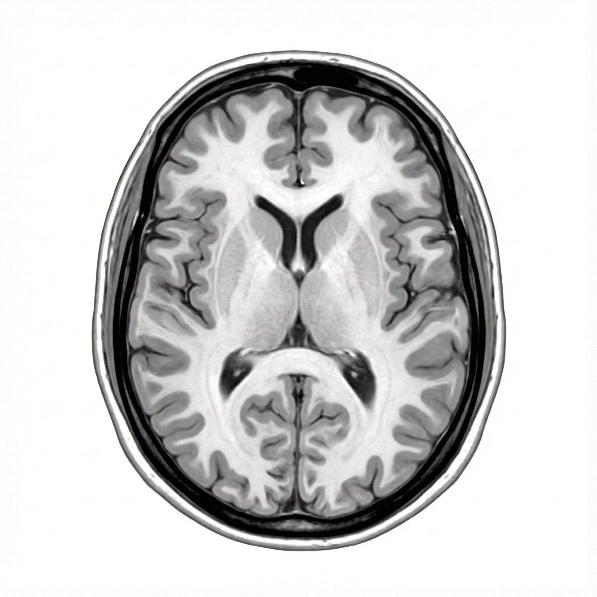
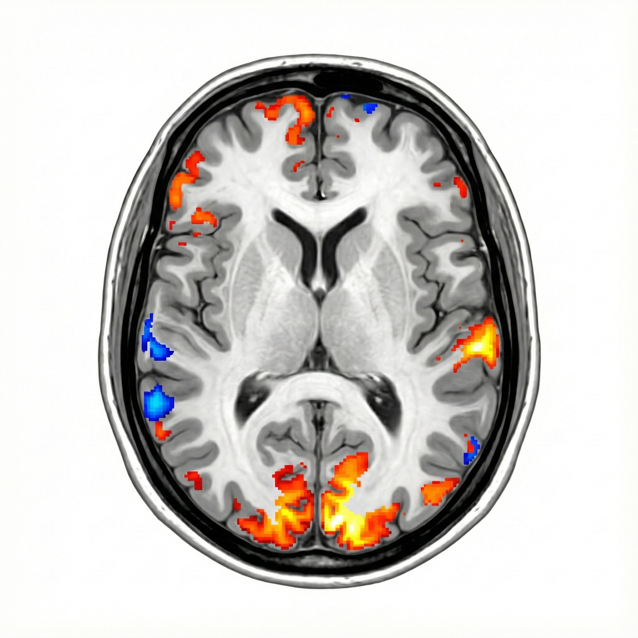
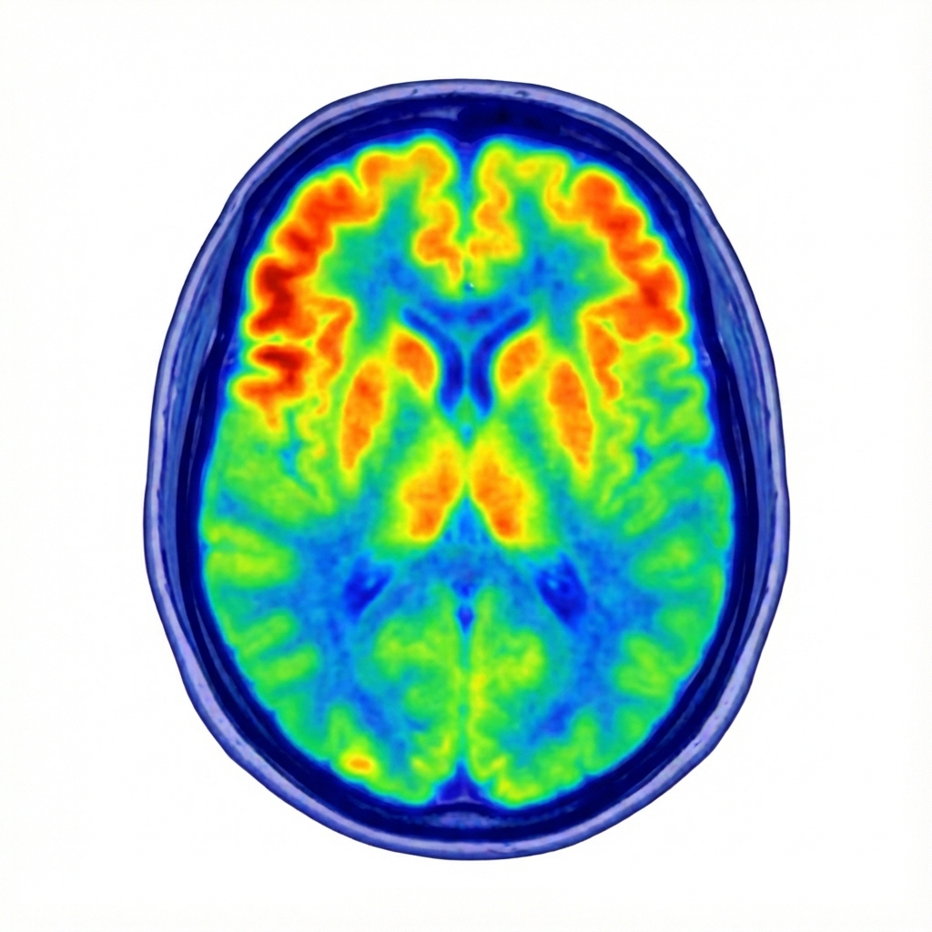
Biomedical imaging

MRI: structural
fMRI: functional
PET: metabolic
Clinical notes

MRI

fMRI

PET

Notes

5 / 23

AI / ML Imputation: Imaging

Advanced vision models can generate missing imaging modalities from the observed ones.
Advanced language models can produce doctor notes from any available imaging.
AI generation comes with no built-in quality control.

MRI

fMRI

PET

Notes

6 / 23

Multi-Modality Data: Single-Cell Sequencing

Single-cell sequencing

RNA-seq: gene expression
ATAC-seq: chromatin accessibility
Proteomics: protein abundance

RNA-seq

ATAC-seq

Proteomics

7 / 23

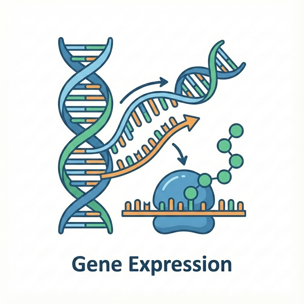
AI / ML Imputation: Single Cell

Advanced single-cell foundation models can impute missing sequencing modalities.
Model-based predictions can still deviate substantially from the true measurements.

RNA-seq

ATAC-seq

Proteomics

8 / 23

Problem Setup: Data and Patterns

Complete data: $p$ modalities, $Z=(X_1,\ldots,X_p)\sim\mathcal{P}_Z$.
$\mathcal{Q}\subseteq 2^{[p]}$ collects all observed patterns.
Random variable $R\in\mathcal{Q}$ indicates the observed pattern.
$Z_r=(X_j)_{j\in r},\ r\in\mathcal{Q}$.
Sample size $n_r$ and population proportion $\pi_r$.

$X_1$

$X_2$

$Y$

$R=\{1,2,3\}$$\pi_{123}$

$n_{123}$

$R=\{1,2\}$$\pi_{12}$

$n_{12}$

$R=\{1,3\}$$\pi_{13}$

$n_{13}$

$R=\{1\}$$\pi_1$

$n_1$

$\mathcal{Q}=\{\{1,2,3\},\{1,2\},\{1,3\},\{1\}\}$

9 / 23

Problem Setup: Assumptions and Target Parameters

Missing mechanism: MCAR (this talk) or MAR (next arXiv version).
Positivity: $\pi_{[p]} > 0$.
Target parameter: regular estimand $\theta^*$.

$\mathbb{E}\{\varphi(Z,\theta^*)\}=0$

$\theta^*=\mathbb{E}[Y]$$\theta^*=\mathrm{quantile}(Y,\tau)$$\theta^*=\beta_j$ in a regression of $Y$ on $(X_1,X_2)$

$X_1$

$X_2$

$Y$

10 / 23

Literature Review

Naive estimator: use complete data to estimate $\theta^*$.
Prediction-powered inference: semi-supervised setting. (Angelopoulos et al., 2023a; PPI++: Angelopoulos et al., 2023b)
Imputation-powered inference / pattern-stratified PPI: blockwise missing setting. (Zhao and Candès, 2025; Chen et al., 2025; Duan and Pelger, 2025)
Existing estimators are unbiased and consistent.
They are not semiparametric efficient, even with perfect AI/ML imputation.
Question: Can we attain the efficiency lower bound under blockwise missingness and MCAR?

$X_1$

$X_2$

$Y$

11 / 23

Optimal Estimating Equation

Optimal estimating equation (Robins et al., 1994):

$\mathcal{L}[\mathcal{M}^{-1}(\varphi)] = 0$

Neumann series: $\mathcal{M}^{-1}=\sum_{k=0}^{\infty}(\mathcal{I}-\mathcal{M})^k$.
Neumann expansion creates repeated compositions of conditional expectations.
$\mathcal{M}^k(\cdot)=\sum_{r_1,\ldots,r_k\in\mathcal{Q}}\pi_{r_1}\cdots\pi_{r_k}\mathcal{A}_{r_1}\circ\cdots\circ\mathcal{A}_{r_k}(\cdot)$
These compositions scale over observed patterns and become computationally intractable.

$\mathcal{A}_r(\cdot)=\mathbb{E}[\cdot\mid Z_r]$$\mathcal{M}=\sum_{r\in\mathcal{Q}}\pi_r\mathcal{A}_r(\cdot)$$\mathcal{L}=\sum_{r\in\mathcal{Q}}\mathbb{I}(R=r)\mathcal{A}_r(\cdot)$

Theory

Optimal estimating equation was established.

The solution attains the semiparametric efficiency lower bound.

Computation

High-order conditional-expectation compositions are computationally intractable.

Balance?

EfficiencyFeasibility

12 / 23

Outline of Our Solution

Almost-eigen decomposition of $\mathcal{M}$Approximate $\mathcal{M}^{-1}$ with conditional expectations $\mathcal{A}_r$.
RAY estimatorMotivated by the almost-eigen decomposition.
Generalized RAY spaceA tractable class containing RAY, IPI, and PPI.
Adaptive RAY estimatorThe most efficient estimator within generalized RAY space.

13 / 23

Two New Mathematical Tools

Tool 1

Almost-eigen-operator

$\mathcal{M}(\mathcal{A}_s)=\lambda_s\mathcal{A}_s+\mathrm{Remainder}_s$

$\mathcal{M}(\mathcal{A}_s)\approx\lambda_s\mathcal{A}_s$

Tool 2

RAY decomposition

$\varphi=\sum_{s\subseteq[p]}\mathcal{P}_s(\varphi)$

combining into ...

$\mathcal{M}^{-1}(\varphi) \approx \sum_{s\subseteq[p]}\lambda_s^{-1}\mathcal{P}_s(\varphi)$

$\mathcal{M}=\sum_{r\in\mathcal{Q}}\pi_r\mathcal{A}_r$$\mathcal{A}_s(\cdot)=\mathbb{E}[\cdot\mid Z_s]$$\lambda_s=\sum_{r\supseteq s,\ r\in\mathcal{Q}}\pi_r$$\mathcal{P}_s(\varphi)=\sum_{r\subseteq s,\ r\in\mathcal{Q}}(-1)^{|s|-|r|}\mathcal{A}_r(\varphi)$

14 / 23

RAY estimator

RAY approximation

$\mathcal{L}[\mathcal{M}^{-1}(\varphi)] \approx$$\frac{\mathbb{I}(R=[p])}{\pi_{[p]}}\varphi$$+$$\sum_{r\in\mathcal{Q}, r\neq[p]}\omega_r\mathcal{A}_r(\varphi)$$:=\varphi_{RAY}$

RAY estimator

$\sum_{i=1}^{N}\{$$\frac{\mathbb{I}(R_i=[p])}{\hat{\pi}_{[p]}}\varphi(Z_i,\theta)$$+$$\sum_{r\in\mathcal{Q}, r\neq[p]}\hat{\omega}_{ir}\widehat{\mathbb{E}}[\varphi(Z_i,\theta)\mid Z_{ir}]$$\}=0$

IPW term uses complete cases.
Augmentation terms use conditional expectations from incomplete patterns.
RAY approximation is a valid estimating function for $\theta^*$: $\mathbb{E}[\varphi_{RAY}]=0$.

RAY estimator is unbiased and consistent.
RAY estimator is multiple robust: remains unbiased and consistent even when conditional expectation models are misspecified.
Any AI/ML imputation model $f_r:Z_r\to\mathbb{R}^{\dim(\theta^*)}$ can be plugged in.
RAY estimator is asymptotically normal.

15 / 23

Safeguard Tuning

With biased AI models, RAY can be less efficient than IPW.
Solution: Add safeguard tuning parameters $\alpha_r$ for each AI model $f_r$.

$\varphi_{RAY,\alpha}=\frac{\mathbb{I}(R=[p])}{\pi_{[p]}}\varphi + \sum_{r\in\mathcal{Q},r\neq[p]}\alpha_r\omega_r f_r(Z_r)$

If $f_r$ is non-informative, set $\alpha_r\approx0$.
Choose optimal $\alpha_r$ by minimizing asymptotic variance, which attains at least the same efficiency as IPW.

16 / 23

Is RAY Uniformly More Efficient?

RAYIPIPPI++Naive

17 / 23

Intuition of RAY Estimator

Pretrained models

f$f(X_1)\to Y$

g$g(X_1,X_2)\to Y$

Naivecomplete cases only0

PPI++one model $f$, every pattern4

IPIpattern-stratified4

RAYevery model × every usable pattern6

RAY applies every model wherever it can.

Why is RAY not uniformly more efficient?

18 / 23

RAY, PPI, and IPI Weighting

fWeights of applying $f\!:X_1\to Y$ to each pattern

Observed pattern

RAY

PPI

IPI

X₁X₂Y

$\alpha_1-\frac{\alpha_1}{\pi_{123}+\pi_{12}}-\frac{\alpha_1}{\pi_{123}+\pi_{13}}+\frac{\alpha_1}{\pi_{123}}$

$-\frac{\alpha_1}{\pi_{123}+\pi_{13}}$

$-\frac{\alpha_1}{\pi_{123}}$

X₁X₂

$\alpha_1-\frac{\alpha_1}{\pi_{123}+\pi_{12}}$

$\frac{\alpha_1}{\pi_{12}+\pi_1}$

$0$

X₁Y

$\alpha_1-\frac{\alpha_1}{\pi_{123}+\pi_{13}}$

$-\frac{\alpha_1}{\pi_{123}+\pi_{13}}$

$0$

X₁

$\alpha_1$

$\frac{\alpha_1}{\pi_{12}+\pi_1}$

$\frac{\alpha_1}{\pi_1}$

gWeights of applying $g\!:X_1,X_2\to Y$ to each patternonly patterns with $X_1,X_2$

Observed pattern

RAY

PPI

IPI

X₁X₂Y

$\frac{\alpha_{12}}{\pi_{123}+\pi_{12}}-\frac{\alpha_{12}}{\pi_{123}}$

$0$

$-\frac{\alpha_{12}}{\pi_{123}}$

X₁X₂

$\frac{\alpha_{12}}{\pi_{123}+\pi_{12}}$

$0$

$\frac{\alpha_{12}}{\pi_{12}}$

Does RAY find the optimal weights?

19 / 23

Generalized RAY Space

Unified estimating equation

$\frac{\mathbb{I}(R=[p])}{\pi_{[p]}}\varphi + \sum_{r\in\mathcal{Q},r\neq[p]}\omega_r f_r(Z_r)$

$\omega_r=\sum_{s\supseteq r}\frac{\mathbb{I}(R=s)}{\pi_s}\alpha_{r,s}$, subject to $\sum_{s\supseteq r}\alpha_{r,s}=0$.
$\mathbb{E}[\omega_r]=0$ guarantees unbiasedness, consistency, and multiple robustness.
RAY, PPI, and IPI estimators are special cases in this space.
$f_r$ is applied to all observed patterns containing $r$ with different weights.

20 / 23

Adaptive RAY Estimator

Generalized RAY space is a convex subspace.
The most efficient estimator within the generalized RAY space is the Adaptive RAY estimator.

21 / 23

Simulation: Outcome Mean Estimation

Adaptive RAYRAYIPIPPI++Naive

22 / 23

Summary and Beyond

Summary

Approximate an intractable operator inversion with conditional expectations.
A multiply-robust estimator that plugs in any AI/ML imputation model.
Adaptive RAY achieves an efficiency–feasibility trade-off.

Beyond

Sufficient and necessary conditions for exact approximation.
Estimation and inference under missing at random (MAR).
Efficiency gap between the RAY approximation and the lower bound.

Motivated by emerging AI/ML models, we address a longstanding problem with new mathematical tools.

23 / 23